![]()
The pivottabler package enables pivot tables to be created with just a few lines of R.
The pivottabler package aims to:
- Provide an easy way of creating pivot tables, without requiring the user to specify low-level layout logic.
- Provide multiple ways of specifying calculation logic to cover both simple and more sophisticated requirements.
- Provide styling options so the pivot tables can be themed/branded as needed.
All calculations for the pivot tables take place inside R, enabling the use of a wide-range of R functions in the calculation logic.
Pivot tables are rendered as htmlwidgets, Latex or plain text. The HTML/Latex/text can be exported for use outside of R.
Pivot tables can be converted to a standard R matrix or data frame. Pivot tables can be exported to Excel. Pivot tables can also be converted to a basictabler table for further manipulation.
Using the flextabler package it is also possible to output tables to Word and PowerPoint.
pivottabler is a companion package to the basictabler package. pivottabler is focussed on generating pivot tables and can aggregate data. basictabler does not aggregate data but offers more control of table structure.
For more detailed information see http://www.pivottabler.org.uk/articles.
Installation
You can install:
- the latest released version from CRAN with
install.packages("pivottabler")- the latest development version from GitHub with
devtools::install_github("cbailiss/pivottabler", build_vignettes = TRUE)Example
pivottabler has many styling and formatting capabilities when rendering pivot tables in HTML / as htmlwidgets using pt$renderPivot(), however the most basic output is simply as plain text.
Plain Text Output
A simple example of creating a pivot table - summarising the types of trains run by different train companies:
library(pivottabler)
# arguments: qpvt(dataFrame, rows, columns, calculations, ...)
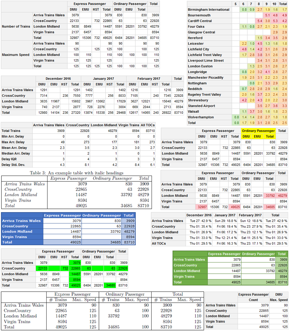
qpvt(bhmtrains, "TOC", "TrainCategory", "n()") # TOC = Train Operating Company Express Passenger Ordinary Passenger Total
Arriva Trains Wales 3079 830 3909
CrossCountry 22865 63 22928
London Midland 14487 33792 48279
Virgin Trains 8594 8594
Total 49025 34685 83710 pivottabler also offers a more verbose syntax that is more self-describing and offers additional options that aren’t available with the quick-pivot functions. The equivalent verbose commands to output the same pivot table as above are:
library(pivottabler)
pt <- PivotTable$new()
pt$addData(bhmtrains) # bhmtrains is a data frame with columns TrainCategory, TOC, etc.
pt$addColumnDataGroups("TrainCategory") # e.g. Express Passenger
pt$addRowDataGroups("TOC") # TOC = Train Operating Company e.g. Arriva Trains Wales
pt$defineCalculation(calculationName="TotalTrains", summariseExpression="n()")
pt$evaluatePivot()
pt
Multiple levels can be added to the pivot table row or column headings, e.g. looking at combinations of TOC and PowerType:
library(pivottabler)
qpvt(bhmtrains, c("TOC", "PowerType"), "TrainCategory", "n()")
library(pivottabler)
pt <- PivotTable$new()
pt$addData(bhmtrains)
pt$addColumnDataGroups("TrainCategory")
pt$addRowDataGroups("TOC")
pt$addRowDataGroups("PowerType") # D/EMU = Diesel/Electric Multiple Unit, HST=High Speed Train
pt$defineCalculation(calculationName="TotalTrains", summariseExpression="n()")
pt$evaluatePivot()
pt
Express Passenger Ordinary Passenger Total
Arriva Trains Wales DMU 3079 830 3909
Total 3079 830 3909
CrossCountry DMU 22133 63 22196
HST 732 732
Total 22865 63 22928
London Midland DMU 5638 5591 11229
EMU 8849 28201 37050
Total 14487 33792 48279
Virgin Trains DMU 2137 2137
EMU 6457 6457
Total 8594 8594
Total 49025 34685 83710 HTML Output
The HTML rendering of the same two pivot tables shown above (each constructed using both a quick-pivot function and verbose syntax) is:
library(pivottabler)
qhpvt(bhmtrains, "TOC", "TrainCategory", "n()")
library(pivottabler)
pt <- PivotTable$new()
pt$addData(bhmtrains)
pt$addColumnDataGroups("TrainCategory")
pt$addRowDataGroups("TOC")
pt$defineCalculation(calculationName="TotalTrains", summariseExpression="n()")
pt$renderPivot()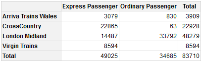
library(pivottabler)
qhpvt(bhmtrains, c("TOC", "PowerType"), "TrainCategory", "n()")
library(pivottabler)
pt <- PivotTable$new()
pt$addData(bhmtrains) # bhmtrains is a data frame with columns TrainCategory, TOC, etc.
pt$addColumnDataGroups("TrainCategory") # e.g. Express Passenger
pt$addRowDataGroups("TOC") # TOC = Train Operating Company e.g. Arriva Trains Wales
pt$addRowDataGroups("PowerType") # D/EMU = Diesel/Electric Multiple Unit, HST=High Speed Train
pt$defineCalculation(calculationName="TotalTrains", summariseExpression="n()")
pt$renderPivot()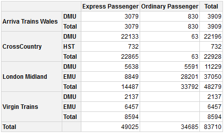
Outline layout is an alternative way of rendering the row groups, e.g. for the same pivot table as above:
library(pivottabler)
pt <- PivotTable$new()
pt$addData(bhmtrains)
pt$addColumnDataGroups("TrainCategory")
pt$addRowDataGroups("TOC",
                    outlineBefore=list(isEmpty=FALSE, groupStyleDeclarations=list(color="blue")),
                    outlineTotal=list(isEmpty=FALSE, groupStyleDeclarations=list(color="blue")))
pt$addRowDataGroups("PowerType", addTotal=FALSE)
pt$defineCalculation(calculationName="TotalTrains", summariseExpression="n()")
pt$renderPivot()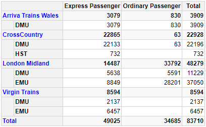
Outline layout can also be used to build a pivot table with a variable depth hierarchy on the rows, e.g. a simple balance sheet:
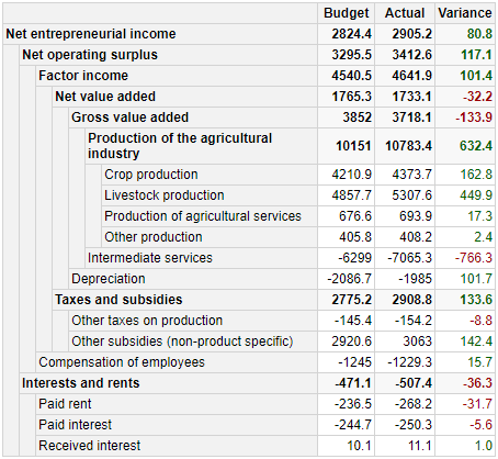
The R for generating the above pivot table can be found in the Regular Layout vignette at http://www.pivottabler.org.uk/articles.
Multiple Calculations
Multiple calculations are supported. Calculations can be based on other calculations in the pivot table. Calculations can be hidden - e.g. to hide calculations that only exist to provide values to other calculations.
For example, looking at the total number of trains and the percentage of trains that arrive more than five minutes late for combinations of train operating company (TOC) and train category:
library(pivottabler)
library(dplyr)
library(lubridate)

# derive train delay data
trains <- mutate(bhmtrains,
                 ArrivalDelta=difftime(ActualArrival, GbttArrival, units="mins"),
                 ArrivalDelay=ifelse(ArrivalDelta<0, 0, ArrivalDelta),
                 DelayedByMoreThan5Minutes=ifelse(ArrivalDelay>=5,1,0))

# create the pivot table
pt <- PivotTable$new()
pt$addData(trains)
pt$addRowDataGroups("TOC", totalCaption="All TOCs")
pt$addColumnDataGroups("TrainCategory", totalCaption="All Trains")
pt$defineCalculation(calculationName="TotalTrains", caption="Train Count",
                     summariseExpression="n()")
pt$defineCalculation(calculationName="DelayedTrains", caption="Trains Arr. 5+ Mins Late",
                     summariseExpression="sum(DelayedByMoreThan5Minutes, na.rm=TRUE)",
                     visible=FALSE)
pt$defineCalculation(calculationName="DelayedPercent", caption="% Late Trains",
                     type="calculation", basedOn=c("DelayedTrains", "TotalTrains"),
                     format="%.1f %%",
                     calculationExpression="values$DelayedTrains/values$TotalTrains*100")
pt$renderPivot()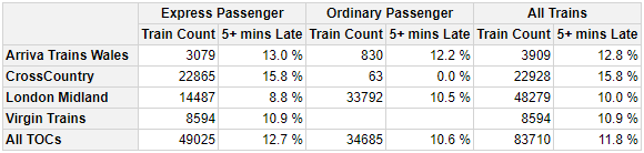
It is also possible to change the axis (rows or columns) and level in which the calculations appear. See the “Calculations” vignette for details.
More advanced calculations such as % of row total, cumulative sums, etc are possible. See the “A2. Appendix: Calculations” vignette for details.
Styling Example
Styling can be specified when creating the pivot table. The example below shows specifying styling using a quick-pivot function and using the more verbose syntax.
library(pivottabler)
qhpvt(bhmtrains, "TOC", "TrainCategory", "n()",
      tableStyle=list("border-color"="maroon"),
      headingStyle=list("color"="cornsilk", "background-color"="maroon",
                        "font-style"="italic", "border-color"="maroon"),
      cellStyle=list("color"="maroon", "background-color"="cornsilk",
                     "border-color"="maroon"),
      totalStyle=list("color"="maroon", "background-color"="cornsilk",
                      "border-color"="maroon", "font-weight"="bold"))
library(pivottabler)
pt <- PivotTable$new(tableStyle=list("border-color"="maroon"),
                     headingStyle=list("color"="cornsilk", "background-color"="maroon",
                                       "font-style"="italic", "border-color"="maroon"),
                     cellStyle=list("color"="maroon", "background-color"="cornsilk",
                                    "border-color"="maroon"),
                     totalStyle=list("color"="maroon", "background-color"="cornsilk",
                                     "border-color"="maroon", "font-weight"="bold"))
pt$addData(bhmtrains)
pt$addColumnDataGroups("TrainCategory")
pt$addRowDataGroups("TOC")
pt$defineCalculation(calculationName="TotalTrains", summariseExpression="n()")
pt$renderPivot()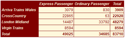
It is also possible to change the styling of single cells and ranges of cells after the pivot table has been created. See the “Styling” and “Finding and Formatting” vignettes for more details.
Excel Output
The same styling/formatting used for the HTML output is also used when outputting to Excel - greatly reducing the amount of script that needs to be written to create Excel output.
library(pivottabler)
pt <- PivotTable$new()
pt$addData(bhmtrains) # bhmtrains is a data frame with columns TrainCategory, TOC, etc.
pt$addColumnDataGroups("TrainCategory") # e.g. Express Passenger
pt$addRowDataGroups("TOC") # TOC = Train Operating Company e.g. Arriva Trains Wales
pt$addRowDataGroups("PowerType") # D/EMU = Diesel/Electric Multiple Unit, HST=High Speed Train
pt$defineCalculation(calculationName="TotalTrains", summariseExpression="n()")
pt$evaluatePivot()

library(openxlsx)
wb <- createWorkbook(creator = Sys.getenv("USERNAME"))
addWorksheet(wb, "Data")
pt$writeToExcelWorksheet(wb=wb, wsName="Data",
                         topRowNumber=2, leftMostColumnNumber=2, applyStyles=TRUE)
saveWorkbook(wb, file="C:\\test.xlsx", overwrite = TRUE)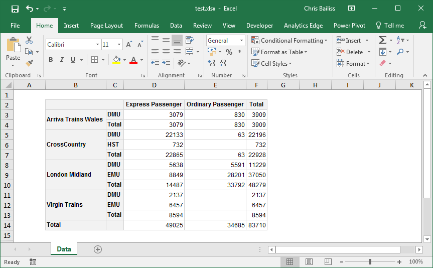
In the screenshot above, Gridlines have been made invisible to make the styling easier to see (by clearing the checkbox on the ‘View’ ribbon). Columns were also auto-sized - though the widths of columns could also be manually specified from R. See the Excel Export vignette for more details.
More Information
More complex pivot tables can also be created, e.g. with irregular layouts, using multiple data frames, using multiple calculations and/or custom R calculation functions.
See http://www.pivottabler.org.uk/articles for more detailed information.