01. Introduction
Chris Bailiss
2023-10-01
Source:vignettes/v01-introduction.Rmd
v01-introduction.RmdIn This Vignette
- Introducing pivottabler
- Pivot Tables
- Quick Example
- Definition
- In reality
- Sample Data
- Basic Pivot Table
- Constructing the Basic Pivot Table
- Outputting the Pivot Table as Plain Text
- Extending the Basic Pivot Table
- Outline Layout
- Quick-Pivot Functions
- Examples Gallery
- Further Reading
Introducing pivottabler
The pivottabler package enables pivot tables to be
created and rendered/exported with just a few lines of R.
Pivot tables are constructed natively in R, either via a short one line command to build a basic pivot table or via series of R commands that gradually build a more bespoke pivot table to meet your needs.
The pivottabler package:
- provides a simple framework for specifying and aggregating data,
based on either the dplyr package or the data.table package.
- provides optional hooks for specifying custom
calculations/aggregations for more complex scenarios
- This allows a wide-range of R functions, including custom functions written in R, to be used in the calculation logic.
- does not require the user to specify low-level layout logic.
- supports output in multiple formats as well as converting a pivot table to either a standard R matrix or data frame.
Since pivot tables are primarily visualisation tools, the pivottabler package offers several custom styling options as well as conditional/custom formatting capabilities so that the pivot tables can be themed/branded as needed.
Output can be rendered as:
- HTML, including via the htmlwidgets framework,
- Latex, e.g. to PDF, or
- Plain text, e.g. to the console.
The generated HTML, Latex and text can also be easily retrieved, e.g. to be used outside of R
The pivot tables can also be exported to Excel, including the styling/formatting.
pivottabler is a companion package to the
basictabler package. pivottabler is focussed
on generating pivot tables and can aggregate data.
basictabler does not aggregate data but offers more control
of table structure.
The latest version of the pivottabler package can be obtained directly from the package repository. Please log any questions not answered by the vignettes or any bug reports here.
Pivot Tables
Quick Example
An example of a pivot table showing the number of trains operated by different train companies is:
library(pivottabler)
# arguments:  qhpvt(dataFrame, rows, columns, calculations, ...)
qhpvt(bhmtrains, "TOC", "TrainCategory", "n()") # TOC = Train Operating Company
This example pivot table is explained in more detail later in this vignette.
Examples of pivot tables containing other types of calculation can be found in the examples gallery later in the vignette.
Definition
Pivot tables are a common technique for summarising large tables of data into smaller and more easily understood summary tables to answer specific questions.
Starting from a specific question that requires answering, the variables relevant to the question are identified. The distinct values of the fixed variables1 are rendered as a mixture of row and column headings in the summary table. One or more aggregations of the (numerical) measured variables are added into the body of the table, where the row/column headings act as data groups. The summary table should then yield an answer to the original question.
In reality
The definition above is probably more difficult to understand than just looking at some examples - several are presented in this vignette. An extended definition is also provided by Wikipedia.
Pivot tables can be found in everyday use within many commercial and non-commercial organisations. Pivot tables feature prominently in applications such as Microsoft Excel, Open Office, etc. More advanced forms are found in Business Intelligence (BI) and Online Analytical Processing (OLAP) tools.
Sample Data: Trains in Birmingham
To build a series of example pivot tables, we will use the
bhmtrains data frame. This contains all 83,710 trains that
arrived into and/or departed from Birmingham
New Street railway station between 1st December 2016 and 28th
February 2017. As an example, the following are four trains that arrived
into Birmingham New Street at the very start of this time period - note
the data has been transposed (otherwise the table would be very
wide).
GbttArrival and GbttDeparture are the scheduled arrival and departure
times of the trains at Birmingham New Street, as advertised in the Great
Britain Train Timetable (GBTT). Also given are the actual arrival and
departure times of the trains at Birmingham New Street. Note that all
four of the trains above terminated at New Street, hence they have
arrival times but no departure times. The origin and destination
stations of each of the trains is also included, in the form of three
letter station codes, e.g. BHM = Birmingham New Street. The
trainstations data frame (used later in this vignette)
includes a lookup from the code to the full station name for all
stations.
The first train above:
- has an identifier of 339607252.
- was operated by the London Midland train operating company.
- was an express passenger train (=fewer stops).
- was scheduled to be operated by an “Electric Multiple Unit”.
- had a scheduled maximum speed of 100mph.
- originated at London Euston station.
- was scheduled to leave Euston at 21:49 on 30th November 2016.
- left on-time (i.e. at 21:49).
- was scheduled to arrive at Birmingham New Street at 00:04 on 1st December 2016.
- arrived on-time at New Street.
- terminated at New Street (so no departure details and the destination was Birmingham New Street).
Basic Pivot Table
Suppose we want to answer the question: How many ordinary/express passenger trains did each train operating company (TOC) operate in the three month period?
The following code will generate the relevant pivot table:
library(pivottabler)
pt <- PivotTable$new()
pt$addData(bhmtrains)
pt$addColumnDataGroups("TrainCategory")
pt$addRowDataGroups("TOC")
pt$defineCalculation(calculationName="TotalTrains", summariseExpression="n()")
pt$renderPivot()
The code above is the verbose version of the quick-pivot example near
the start of this vignette (which used the qhpvt()
function). Both produce the same pivot table and output, but the verbose
version helps more clearly explain the steps involved in constructing
the pivot table.
Each line above works as follows:
- Load the namespace of the pivottabler library.
- Create a new pivot table instance3.
- Specify the data frame that contains the data for the pivot table.
- Add the distinct values from the TrainCategory column in the data frame as columns in the pivot table.
- Add the distinct values from the TOC column in the data frame as rows in the pivot table.
- Specify the calculation. The summarise expression must be an
expression that can be used with the dplyr summarise() function. This
expression is used internally by the pivottabler package with the dplyr
summarise function.
pivottableralso supports data.table - see the Performance vignette for more details. - Generate the pivot table.
Constructing the Basic Pivot Table
The following examples show how each line in the above example constructs the pivot table. To improve readability, each code change is highlighted.
# produces no pivot table
library(pivottabler)
pt <- PivotTable$new()
pt$addData(bhmtrains)
pt$renderPivot()
# specify the column headings
library(pivottabler)
pt <- PivotTable$new()
pt$addData(bhmtrains)
pt$addColumnDataGroups("TrainCategory")   #    << **** LINE ADDED **** <<
pt$renderPivot()
# specify the row headings
library(pivottabler)
pt <- PivotTable$new()
pt$addData(bhmtrains)
pt$addColumnDataGroups("TrainCategory")
pt$addRowDataGroups("TOC")                #    << **** LINE ADDED **** <<
pt$renderPivot()
# specifying a calculation
library(pivottabler)
pt <- PivotTable$new()
pt$addData(bhmtrains)
pt$addColumnDataGroups("TrainCategory")
pt$addRowDataGroups("TOC")                #     **** LINE BELOW ADDED ****
pt$defineCalculation(calculationName="TotalTrains", summariseExpression="n()")
pt$renderPivot()
Outputting the Pivot Table as Plain Text
The pivot table can be rendered as plain text to the console by using
pt:
library(pivottabler)
pt <- PivotTable$new()
pt$addData(bhmtrains)
pt$addColumnDataGroups("TrainCategory")
pt$addRowDataGroups("TOC")
pt$defineCalculation(calculationName="TotalTrains", summariseExpression="n()")
pt$evaluatePivot()
pt
Express Passenger Ordinary Passenger Total
Arriva Trains Wales 3079 830 3909
CrossCountry 22865 63 22928
London Midland 14487 33792 48279
Virgin Trains 8594 8594
Total 49025 34685 83710 Extending the Basic Pivot Table
There follows below a progressive series of changes to the basic pivot table shown above. Each change is made by adding or changing one line of code. Again, to improve readability, each code change is highlighted.
First, adding an additional column data group to sub-divide each “TrainCategory” by “PowerType”:
library(pivottabler)
pt <- PivotTable$new()
pt$addData(bhmtrains)
pt$addColumnDataGroups("TrainCategory")
pt$addColumnDataGroups("PowerType")    #    << **** CODE CHANGE **** <<
pt$addRowDataGroups("TOC")
pt$defineCalculation(calculationName="TotalTrains", summariseExpression="n()")
pt$renderPivot()
By default, the new data group does not expand the existing “TrainCategory” total. However, an additional argument allows the total column to also be expanded:
library(pivottabler)
pt <- PivotTable$new()
pt$addData(bhmtrains)
pt$addColumnDataGroups("TrainCategory")
pt$addColumnDataGroups("PowerType", expandExistingTotals=TRUE) # << ** CODE CHANGE ** <<
pt$addRowDataGroups("TOC")
pt$defineCalculation(calculationName="TotalTrains", summariseExpression="n()")
pt$renderPivot()
Instead of adding “PowerType” as columns, it can also be added as rows:
library(pivottabler)
pt <- PivotTable$new()
pt$addData(bhmtrains)
pt$addColumnDataGroups("TrainCategory")
pt$addRowDataGroups("TOC")
pt$addRowDataGroups("PowerType")    #    << **** CODE CHANGE **** <<
pt$defineCalculation(calculationName="TotalTrains", summariseExpression="n()")
pt$renderPivot()
It is possible to continue adding additional data groups. The pivottabler does not enforce a maximum depth of data groups. For example, adding the maximum scheduled speed to the rows:
library(pivottabler)
pt <- PivotTable$new()
pt$addData(bhmtrains)
pt$addColumnDataGroups("TrainCategory")
pt$addRowDataGroups("TOC")
pt$addRowDataGroups("PowerType")
pt$addRowDataGroups("SchedSpeedMPH")    #    << **** CODE CHANGE **** <<
pt$defineCalculation(calculationName="TotalTrains", summariseExpression="n()")
pt$renderPivot()
As more data groups are added, the pivot table can seem overwhelmed
with totals. It is possible to selectively show/hide totals using the
addTotal argument. Totals can be renamed using the
totalCaption argument. Both of these options are
demonstrated below.
library(pivottabler)
pt <- PivotTable$new()
pt$addData(bhmtrains)
pt$addColumnDataGroups("TrainCategory")
pt$addRowDataGroups("TOC", totalCaption="Grand Total")    #    << **** CODE CHANGE **** <<
pt$addRowDataGroups("PowerType")
pt$addRowDataGroups("SchedSpeedMPH", addTotal=FALSE)      #    << **** CODE CHANGE **** <<
pt$defineCalculation(calculationName="TotalTrains", summariseExpression="n()")
pt$renderPivot()
This can then be rendered in outline layout:
library(pivottabler)
pt <- PivotTable$new()
pt$addData(bhmtrains)
pt$addColumnDataGroups("TrainCategory")
pt$addRowDataGroups("TOC",
outlineBefore=list(isEmpty=FALSE,
groupStyleDeclarations=list(color="blue")),
outlineTotal=list(groupStyleDeclarations=list(color="blue")))
pt$addRowDataGroups("PowerType", addTotal=FALSE)
pt$addRowDataGroups("SchedSpeedMPH", addTotal=FALSE)
pt$defineCalculation(calculationName="TotalTrains", summariseExpression="n()")
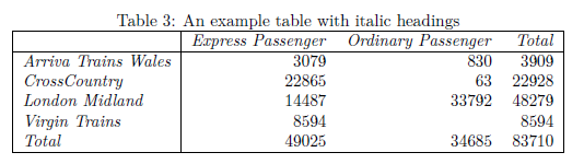
pt$renderPivot()Outline Layout
Outline layout renders row data groups as headings:
library(pivottabler)
pt <- PivotTable$new()
pt$addData(bhmtrains)
pt$addColumnDataGroups("TrainCategory")
pt$addRowDataGroups("TOC",
                    outlineBefore=list(groupStyleDeclarations=list(color="blue")),
                    outlineAfter=list(isEmpty=FALSE,
                                      mergeSpace="dataGroupsOnly",
                                      caption="Total ({value})",
                                      groupStyleDeclarations=list("font-style"="italic")),
                    outlineTotal=list(groupStyleDeclarations=list(color="blue"),
                                      cellStyleDeclarations=list("color"="blue")))
pt$addRowDataGroups("PowerType", addTotal=FALSE)
pt$defineCalculation(calculationName="TotalTrains", summariseExpression="n()")
pt$renderPivot()
Quick-Pivot Functions
To construct basic pivot tables quickly, three functions are provided that can construct pivot tables with one line of R:
-
qpvt()returns a pivot table. Setting a variable equal to the return value, e.g.pt <- qpvt(...), allows further operations to be carried out on the pivot table. Otherwise, usingqpvt(...)alone will simply print the pivot table to the console and then discard it. -
qhpvt()returns a HTML widget that when used alone will render a HTML representation of the pivot table (e.g. in the R-Studio “Viewer” pane). -
qlpvt()returns a Latex representation of a pivot table.
These functions do not offer all of the options that are available when constructing a pivot table using the more verbose syntax.
The arguments to all three functions are essentially the same:
-
dataFramespecifies the data frame that contains the pivot table data. -
rowsspecifies the names of the variables (as a character vector) used to generate the row data groups. -
columnsspecifies the names of the variables (as a character vector) used to generate the column data groups. -
calculationsspecifies the summary calculations (as a character vector) used to calculate the cell values in the pivot table. The names of the elements in this vector become the calculation names (and so the calculation headings when more than one calculation is present in the pivot table). -
formatspecifies the same formatting for all calculations (as either a character value, list or R function). See the “Formatting calculated values” section of the Calculations vignette for more details. -
formatsspecifies a different format for each calculation (as a list of the same length ascalculationscontaining any combination of character values, lists or R functions). -
totalsspecifies which totals are shown and can also control the captions of totals. This is described in more detail below.
Specifying “=” in either the rows or
columns vectors sets the position of the calculations in
the row/column headings.
A basic example of quickly printing a pivot table to the console:
library(pivottabler)
qpvt(bhmtrains, "TOC", "TrainCategory", "n()")
Express Passenger Ordinary Passenger Total
Arriva Trains Wales 3079 830 3909
CrossCountry 22865 63 22928
London Midland 14487 33792 48279
Virgin Trains 8594 8594
Total 49025 34685 83710 A slightly more complex pivot table being quickly rendered as a HTML widget, where the calculation headings are on the rows:
library(pivottabler)
qhpvt(bhmtrains, c("=", "TOC"), c("TrainCategory", "PowerType"),
    c("Number of Trains"="n()", "Maximum Speed"="max(SchedSpeedMPH, na.rm=TRUE)"))
A quick pivot table with a format specified:
library(pivottabler)
qhpvt(bhmtrains, "TOC", "TrainCategory", "mean(SchedSpeedMPH, na.rm=TRUE)", format="%.0f")
A quick pivot table with two calculations that are formatted differently:
library(pivottabler)
qhpvt(bhmtrains, "TOC", "TrainCategory",
     c("Mean Speed"="mean(SchedSpeedMPH, na.rm=TRUE)", "Std Dev Speed"="sd(SchedSpeedMPH, na.rm=TRUE)"),
     formats=list("%.0f", "%.1f"))
In the above pivot table, the “Total” would be better renamed to something like “All” or “Overall” since a total for a mean or standard deviation does not make complete sense.
Totals can be controlled using the totals argument. This
works as follows:
- If not specified, then totals are generated for all variables.
- To hide all totals, specify
totals=NONE. - To specify which variables have totals, specify the names of the
variables in a character vector, e.g. in a pivot table containing the
variables x, y and z, to display totals only for variables x and z,
specify
totals=c("x", "z"). - To specify which variables have totals and also rename the captions
of the total cells, specify a list, e.g. to rename the totals for x to
“All x” and y to “All y”, specify
totals=list("x"="All x", "y"="All y").
Returning to the previous quick pivot example, the totals can now be renamed to “All …” using:
Examples Gallery
This section shows some examples from the other vignettes as a quick overview of some of the other capabilities of the pivottabler package. The R scripts to create each example below can be found in the other vignettes.
Multiple Levels & Formatted Data Groups
See the Data Groups vignette for more details.
Multiple Calculations & Calculations on Rows
See the Calculations vignette for more details.
Custom Calculations
See the Calculations vignette for more details.
Outline Layout
See the Regular Layout vignette for more details.
Results as a Matrix
                      DMU   EMU HST Total
Arriva Trains Wales  3909    NA  NA  3909
CrossCountry        22196    NA 732 22928
London Midland      11229 37050  NA 48279
Virgin Trains        2137  6457  NA  8594
Total               39471 43507 732 83710
See the Outputs vignette for more details, including other conversion options such as converting a pivot table to a data frame.
Styling
See the Styling vignette for more details.
Finding and Formatting Data Groups
See the Finding and Formatting vignette for more details.
Finding and Formatting Cells
See the Finding and Formatting vignette for more details.
Conditional Formatting
See the Finding and Formatting vignette for more details.
Mixing Data Groups and/or Calculations
See the Irregular Layout vignette for more details.
Combining Pivot Tables
See the Irregular Layout vignette for more details.
The terms “fixed variables” and “measured variables” are used here as in Wickham 2014↩︎
This is the identifier assigned by the Recent Train Times website, the source of this sample data↩︎
pivottabler is implemented in R6 Classes so pt here is an instance of the R6 PivotTable class.↩︎